一. Density Estimation 密度估计
假如要更为正式定义异常检测问题,首先我们有一组从 $x^{(1)}$ 到 $x^{(m)}$ m个样本,且这些样本均为正常的。我们将这些样本数据建立一个模型 p(x) , p(x) 表示为 x 的分布概率。
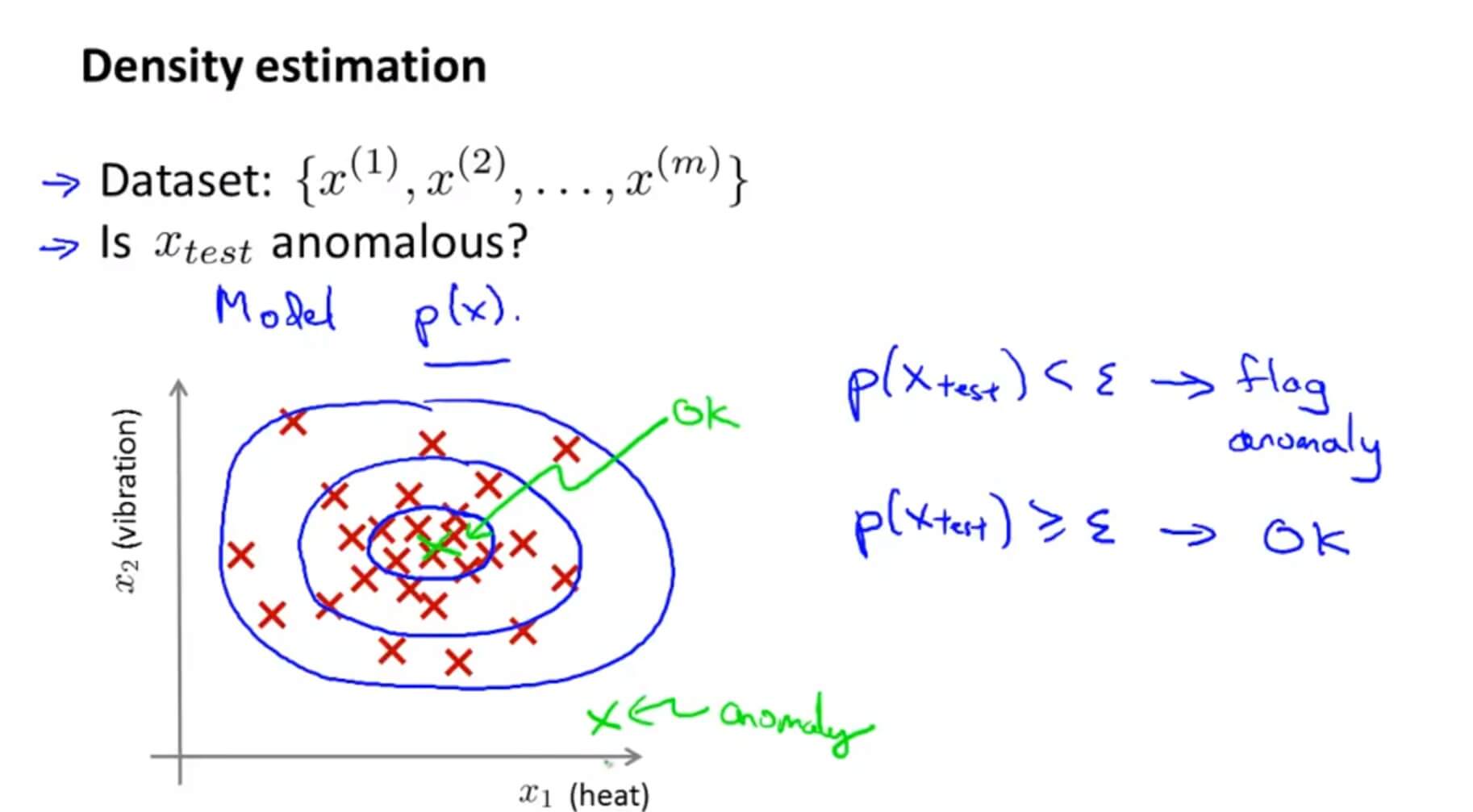
那么假如我们的测试集 $x_{test}$ 概率 p 低于阈值 $\varepsilon$ ,那么则将其标记为异常。
异常检测的核心就在于找到一个概率模型,帮助我们知道一个样本落入正常样本中的概率,从而帮助我们区分正常和异常样本。高斯分布(Gaussian Distribution)模型就是异常检测算法最常使用的概率分布模型。
1. 高斯分布
假如 x 服从高斯分布,那么我们将表示为: $x\sim N(\mu,\sigma^2)$ 。其分布概率为:
$$p(x;\mu,\sigma^2)=\frac{1}{\sqrt{2\pi}\sigma}exp(-\frac{(x-\mu)^2}{2\sigma^2})$$
其中 $\mu$ 为期望值(均值), $\sigma^2$ 为方差。
其中,期望值 $\mu$ 决定了其轴的位置,标准差 $\sigma$ 决定了分布的幅度宽窄。当 $\mu=0,\sigma=1$ 时的正态分布是标准正态分布。
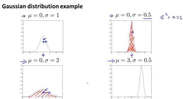
由概率分布的性质,曲线下方的面积等于 1,即积分为 1,所以图形越宽,高度越矮;图像越高,宽度越窄。
期望值:
方差:
上面计算期望值和方差,就是统计学里面的极大似然估计。
假如我们有一组 m 个无标签训练集,其中每个训练数据又有 n 个特征,那么这个训练集应该是 m 个 n 维向量构成的样本矩阵。
在概率论中,对有限个样本进行参数估计
$$\mu_j = \frac{1}{m} \sum_{i=1}^{m}x_j^{(i)}, \;\; \delta^2_j = \frac{1}{m} \sum_{i=1}^{m}(x_j^{(i)}-\mu_j)^2$$
这里对参数 $\mu$ 和参数 $\delta^2$ 的估计就是二者的极大似然估计。
假定每一个特征 $x_{1}$ 到 $x_{n}$ 均服从正态分布,则其模型的概率为:
当 $p(x)<\varepsilon$时,$x$ 为异常样本。
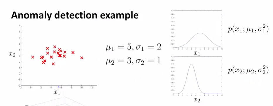
2. 举例
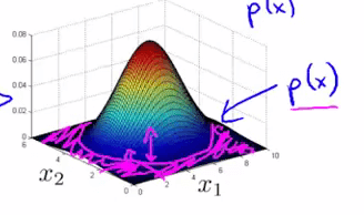
假定我们有两个特征 $x_1$ 、 $x_2$ ,它们都服从于高斯分布,并且通过参数估计,我们知道了分布参数:
则模型 $p(x)$ 能由如下的热力图反映,热力图越热的地方,是正常样本的概率越高,参数 $\varepsilon$ 描述了一个截断高度,当概率落到了截断高度以下(下图紫色区域所示),则为异常样本:
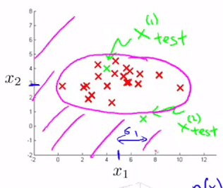
将 $p(x)$ 投影到特征 $x_1$ 、$x_2$ 所在平面,下图紫色曲线就反映了 $\varepsilon$ 的投影,它是一条截断曲线,落在截断曲线以外的样本,都会被认为是异常样本:
3. 算法评估
由于异常样本是非常少的,所以整个数据集是非常偏斜的,我们不能单纯的用预测准确率来评估算法优劣,所以用我们之前的查准率(Precision)和召回率(Recall)计算出 F 值进行衡量异常检测算法了。
- 真阳性、假阳性、真阴性、假阴性
- 查准率(Precision)与 召回率(Recall)
- F1 Score
我们还有一个参数 $\varepsilon$ ,这个 $\varepsilon$ 是我们用来决定什么时候把一个样本当做是异常样本的阈值。我们应该试用多个不同的 $\varepsilon$ 值,选取一个使得 F 值最大的那个 $\varepsilon$ 。
二. Building an Anomaly Detection System
1. 有监督学习与异常检测
| 有监督学习 | 异常检测 |
|---|---|
| 数据分布均匀 | 数据非常偏斜,异常样本数目远小于正常样本数目 |
| 可以根据对正样本的拟合来知道正样本的形态,从而预测新来的样本是否是正样本 | 异常的类型不一,很难根据对现有的异常样本(即正样本)的拟合来判断出异常样本的形态 |
下面的表格则展示了二者的一些应用场景:
| 有监督学习 | 异常检测 |
|---|---|
| 垃圾邮件检测 | 故障检测 |
| 天气预测(预测雨天、晴天、或是多云天气) | 某数据中心对于机器设备的监控 |
| 癌症的分类 | 制造业判断一个零部件是否异常 |
如果异常样本非常少,特征也不一样完全一样(比如今天飞机引擎异常是因为原因一,明天飞机引擎异常是因为原因二,谁也不知道哪天出现异常是什么原因),这种情况下就应该采用异常检测。
如果异常样本多,特征比较稳当,这种情况就应该采用监督学习。
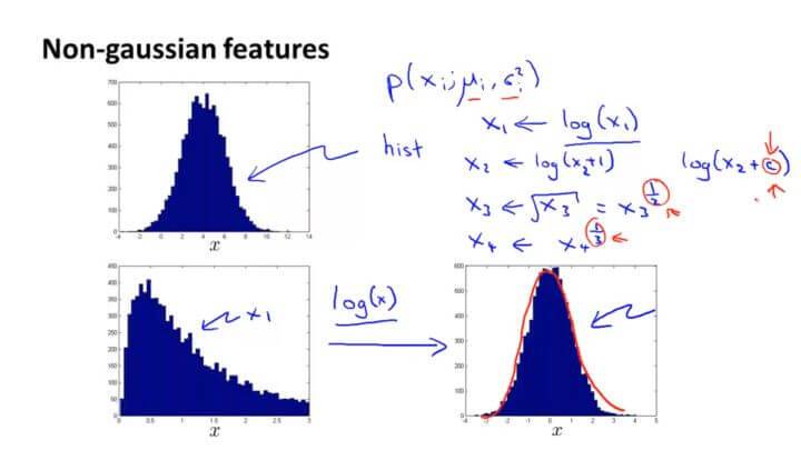
假如我们的数据看起来不是很服从高斯分布,可以通过对数、指数、幂等数学变换让其接近于高斯分布。
三. Multivariate Gaussian Distribution (Optional)
1. 多元高斯分布模型
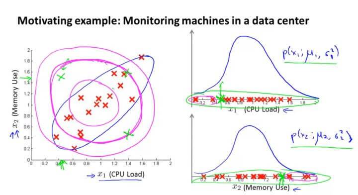
我们以数据中心的监控计算机为例子。 $x_1$ 是CPU的负载,$x_2$ 是内存的使用量。其正常样本如左图红色点所示。假如我们有一个异常的样本(图中左上角绿色点),在图中看很明显它并不是正常样本所在的范围。但是在计算概率 $p(x)$ 的时候,因为它在 $x_1$ 和 $x_2$ 的高斯分布都属于正常范围,所以该点并不会被判断为异常点。
这是因为在高斯分布中,它并不能察觉在蓝色椭圆处才是正常样本概率高的范围,其概率是通过圆圈逐渐向外减小。所以在同一个圆圈内,虽然在计算中概率是一样的,但是在实际上却往往有很大偏差。
所以我们开发了一种改良版的异常检测算法:多元高斯分布。
我们不将每一个特征值都分开进行高斯分布的计算,而是作为整个模型进行高斯分布的拟合。
其概率模型为: $$p(x;\mu,\Sigma)=\frac{1}{(2\pi)^{\frac{n}{2}}|\Sigma|^{\frac{1}{2}}}exp(-\frac{1}{2}(x-\mu)^T\Sigma^{-1}(x-\mu))$$ (其中 $|\Sigma|$ 是 $\Sigma$ 的行列式,$\mu$ 表示样本均值,$\Sigma$ 表示样本协方差矩阵)
多元高斯分布模型的热力图如下:
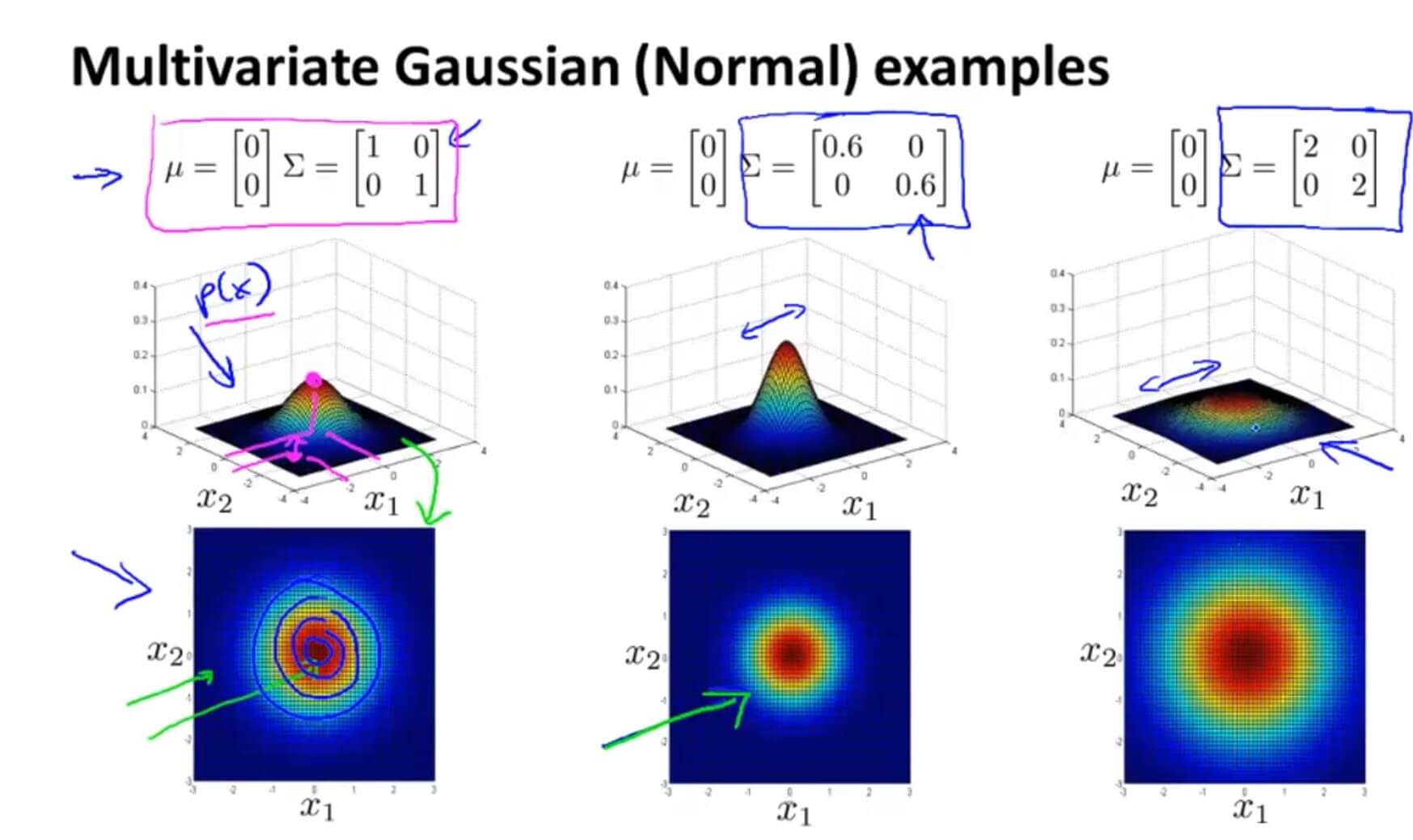
$\Sigma$ 是一个协方差矩阵,所以它衡量的是方差。减小 $\Sigma$ 其宽度也随之减少,增大反之。
同理,多元高斯分布模型也同样遵循概率分布,曲线下方的积分等于 1。如上图,多元高斯分布相当于体积为1 。这样就可以通过 $\mu$ 和 $\Sigma$ (这里是协方差矩阵,原来是 $\sigma$ )的关系来判断图形的大致形状。
$\Sigma$ 中第一个数字是衡量 $x_1$ 的,假如减少第一个数字,则可从图中观察到 $x_1$ 的范围也随之被压缩,变成了一个椭圆。
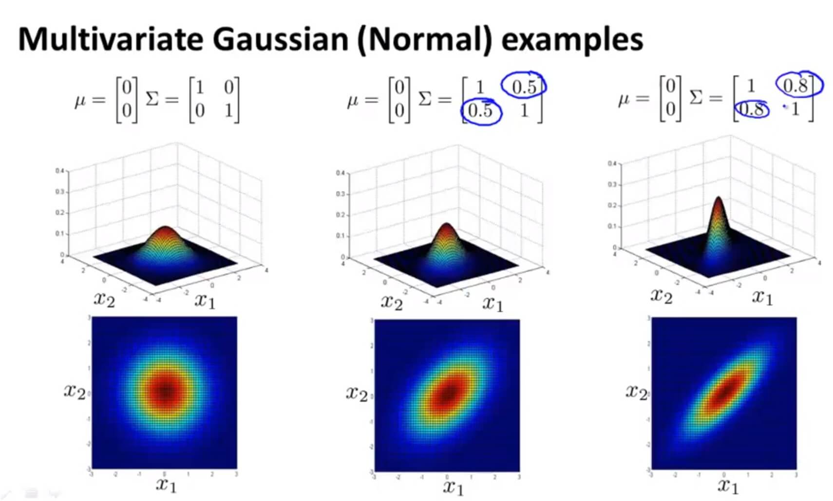
多元高斯分布还可以给数据的相关性建立模型。假如我们在非主对角线上改变数据(如图中间那副),则其图像会根据 $y=x$ 这条直线上进行高斯分布。
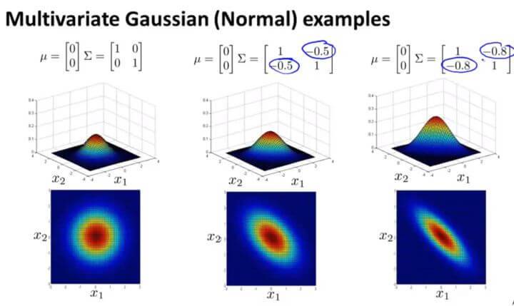
反之亦然。
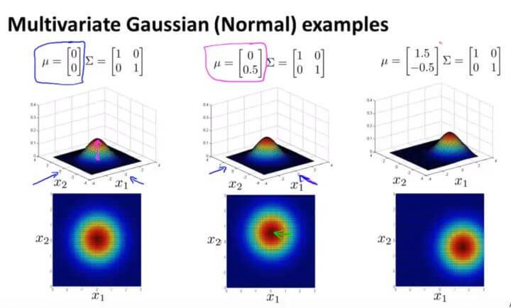
改变 $\mu$ 的值则是改变其中心点的位置。
2. 参数估计
多元高斯分布模型的参数估计如下:
$$\mu=\frac{1}{m}\sum_{i=1}^{m}{x^{(i)}}$$
$$\Sigma=\frac{1}{m}\sum_{i=1}^{m}{(x^{(i)}-\mu)(x^{(i)}-\mu)^T}$$
3. 算法流程
采用了多元高斯分布的异常检测算法流程如下:
- 选择一些足够反映异常样本的特征 $x_j$ 。
- 对各个样本进行参数估计:
$$\mu=\frac{1}{m}\sum_{i=1}^{m}{x^{(i)}}$$
$$\Sigma=\frac{1}{m}\sum_{i=1}^{m}{(x^{(i)}-\mu)(x^{(i)}-\mu)^T}$$ - 当新的样本 x 到来时,计算 $p(x)$ :
$$p(x)=\frac{1}{(2\pi)^{\frac{n}{2}}|\Sigma|^{\frac{1}{2}}}exp(-\frac{1}{2}(x-\mu)^T\Sigma^{-1}(x-\mu))$$
如果 $p(x)<\varepsilon $ ,则认为样本 x 是异常样本。
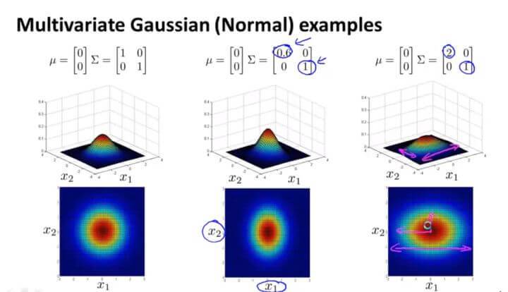
4. 多元高斯分布模型与一般高斯分布模型的差异
一般的高斯分布模型只是多元高斯分布模型的一个约束,它将多元高斯分布的等高线约束到了如下所示同轴分布(概率密度的等高线是沿着轴向的):
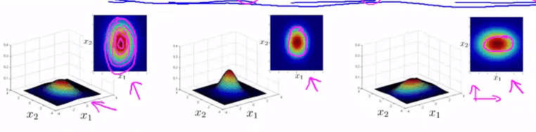
一般的多元高斯模型的轮廓(等高线)总是轴对齐的(axis-aligned),也就是 $\Sigma $ 除对角线以外的部分都是 0,当对角线以外的部分不为 0 的时候,等高线会出现斜着的,与两个轴产生一定的斜率。
当: $\Sigma=\left[ \begin{array}{ccc}\sigma_1^2 \\ & \sigma_2^2 \\ &&…\\&&&\sigma_n^2\end{array} \right]$ 的时候,此时的多元高斯分布即是原来的多元高斯分布。(因为只有主对角线方差,并没有其它斜率的变化)
对比
| 一般高斯模型 | |
|---|---|
| 模型定义 | 见上面公式 |
| 相关性 | 需要手动创建一些特征来描述某些特征的相关性 |
| 复杂度 | 计算复杂度低,适用于高维特征 |
| 效果 | 在样本数目 m 较小时也工作良好 |
| 多元高斯模型 | |
|---|---|
| 模型定义 | 见上面公式 |
| 相关性 | 利用协方差矩阵$\Sigma$获得了各个特征相关性 |
| 复杂度 | 计算复杂 |
| 效果 | 需要 $\Sigma$ 可逆,亦即需要 $m>n$ ,且各个特征不能线性相关,如不能存在 $x_2=3x_1$ 或者 $x_3=x_1+2x_2$ |
结论:基于多元高斯分布模型的异常检测应用十分有限。
四. Anomaly Detection 测试
1. Question 1
For which of the following problems would anomaly detection be a suitable algorithm?
A. Given a dataset of credit card transactions, identify unusual transactions to flag them as possibly fraudulent.
B. Given data from credit card transactions, classify each transaction according to type of purchase (for example: food, transportation, clothing).
C. Given an image of a face, determine whether or not it is the face of a particular famous individual.
D. From a large set of primary care patient records, identify individuals who might have unusual health conditions.
解答:A、D
A、D 才适合异常检测算法。
2. Question 2
Suppose you have trained an anomaly detection system for fraud detection, and your system that flags anomalies when $p(x)$ is less than ε, and you find on the cross-validation set that it is missing many fradulent transactions (i.e., failing to flag them as anomalies). What should you do?
A. Decrease $\varepsilon$
B. Increase $\varepsilon$
解答:B
3. Question 3
Suppose you are developing an anomaly detection system to catch manufacturing defects in airplane engines. You model uses
$$p(x) = \prod_{j=1}^{n}p(x_{j};\mu_{j},\sigma_{j}^{2})$$
You have two features $x_1$ = vibration intensity, and $x_2$ = heat generated. Both $x_1$ and $x_2$ take on values between 0 and 1 (and are strictly greater than 0), and for most "normal" engines you expect that $x_1 \approx x_2$. One of the suspected anomalies is that a flawed engine may vibrate very intensely even without generating much heat (large $x_1$, small $x_2$), even though the particular values of $x_1$ and $x_2$ may not fall outside their typical ranges of values. What additional feature $x_3$ should you create to capture these types of anomalies:
A. $x_3 = \frac{x_1}{x_2}$
B. $x_3 = x_1^2\times x_2^2$
C. $x_3 = (x_1 + x_2)^2$
D. $x_3 = x_1 \times x_2^2$
解答:A
假如特征量 $x_1$ 和 $x_2$ ,可建立特征量 $x_3=\frac{x_1}{x_2}$ 结合两者。
4. Question 4
Which of the following are true? Check all that apply.
A. When evaluating an anomaly detection algorithm on the cross validation set (containing some positive and some negative examples), classification accuracy is usually a good evaluation metric to use.
B. When developing an anomaly detection system, it is often useful to select an appropriate numerical performance metric to evaluate the effectiveness of the learning algorithm.
C. In a typical anomaly detection setting, we have a large number of anomalous examples, and a relatively small number of normal/non-anomalous examples.
D. In anomaly detection, we fit a model p(x) to a set of negative (y=0) examples, without using any positive examples we may have collected of previously observed anomalies.
解答:B、D
5. Question 5
You have a 1-D dataset $\begin{Bmatrix}
x^{(i)},\cdots,x^{(m)}
\end{Bmatrix}$ and you want to detect outliers in the dataset. You first plot the dataset and it looks like this:
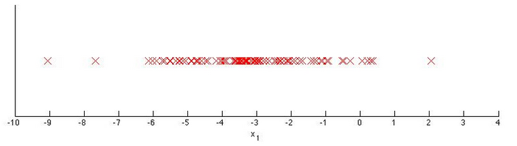
Suppose you fit the gaussian distribution parameters $\mu_1$ and $\sigma_1^2$ to this dataset. Which of the following values for $\mu_1$ and $\sigma_1^2$ might you get?
A. $\mu = -3$,$\sigma_1^2 = 4$
B. $\mu = -6$,$\sigma_1^2 = 4$
C. $\mu = -3$,$\sigma_1^2 = 2$
D. $\mu = -6$,$\sigma_1^2 = 2$
解答:A
中心点在-3,在-3周围即(-4,-2)周围仍比较密集,所以 $\sigma_1=2$ 。
GitHub Repo:Halfrost-Field
Follow: halfrost · GitHub