初探支持向量机

一. 引子

在逻辑回归中，我们的预测函数为：

$$h_\theta(x)=\frac{1}{1+e^{-\theta^Tx}}$$

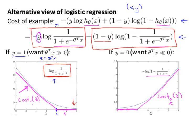
对于每一个样本 (x,y) 而言（注意是每一个），其代价函数为：

$$ \begin{align*} J(\theta)&=-(ylogh_\theta(x)+(1-y)log(1-h_\theta((x)))\\ &=-ylog\frac{1}{1+e^{-\theta^Tx}}-(1-y)log(1-\frac{1}{1+e^{-\theta^Tx}}) \end{align*}\\ $$

那么当 y=1 的时候， $J(\theta)=-ylog\frac{1}{1+e^{-\theta^Tx}}$ ，其代价函数的图像入左下图所示。

当 y=0 的时候， $J(\theta)=-(1-y)log(1-\frac{1}{1+e^{-\theta^Tx}})$ ，其代价函数的图像入右下图所示。

对于支持向量机而言，

$y=1$ 的时候：

$$cost_1(\theta^Tx^{(i)})=(-logh_\theta(x^{(i)}))$$

$y=0$ 的时候：

$$cost_0((\theta^Tx^{(i)})=((-log(1-h_\theta(x^{(i)})))$$

当 y=1 时，随着 z 取值变大，预测代价变小，因此，逻辑回归想要在面对正样本 y=1 时，获得足够高的预测精度，就希望 $z= \theta^Tx\gg 0 $ 。而 SVM 则将上图的曲线拉直为下图中的折线，构成了 y=1 时的代价函数曲线 $cost_1(z)$ ：

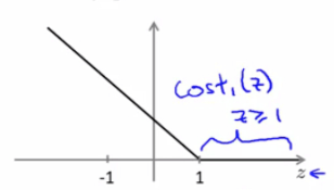
当 y=1 时，为了预测精度足够高，SVM 希望 $\theta^Tx\geqslant 1$ 。

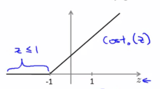
同样，在 y=0 时，SVM 定义了代价函数 $cost_0(z)$ ，为了预测精度足够高，SVM 希望 $\theta^Tx \leqslant -1$ ：

在逻辑回归中，其代价函数是：

$$J(\theta)=min_{\theta} \frac{1}{m}[\sum_{i=1}^{m}{y^{(i)}}(-logh_\theta(x^{(i)}))+(1-y^{(i)})((-log(1-h_\theta(x^{(i)})))]+\frac{\lambda}{2m}\sum_{j=1}^{n}{\theta_j^2}$$

对于逻辑回归而言，其代价函数是有两项决定的，第一项是来自训练样本的代价函数，第二项是正则化项，这就相当于我们用最小化 A 加上正则化参数 $\lambda$ 乘以参数平方项 B，其形式大概是： $A+\lambda B$ 。这里我们是通过设置不同的正则参数 $\lambda$ 来达到优化的目的。但是在支持向量机这里，把参数提到前面，用参数 C 作为 A 的参数，以 A 作为权重。所以其形式是这样的： $CA+B$ 。

在逻辑回归中，我们通过正规化参数 $\lambda$ 调节 A、B 所占的权重，且 A 的权重与$\lambda$ 取值成反比。而在 SVM 中，则通过参数 C 调节 A、B 所占的权重，且 A 的权重与 C 的取值成反比。亦即，参数 C 可以被认为是扮演了 $\frac{1}{\lambda}$ 的角色。

所以 $\frac{1}{ m}$ 这一项仅仅是相当于一个常量，对于最小化参数 $\theta$ 是没有完全任何影响的，所以这里我们将其去掉。

支持向量机的代价函数为：

$$min_{\theta} C[\sum_{i=1}^{m}{y^{(i)}}cost_1(\theta^Tx^{(i)})+(1-y^{(i)})cost_0(\theta^Tx^{(i)})]+\frac{1}{2}\sum_{j=1}^{n}{\theta_j^2}$$

有别于逻辑回归假设函数输出的是概率，支持向量机它是直接预测 y 的值是0还是1。也就是说其假设函数是这样子的：

$$h_{\theta}(x)=\left\{\begin{matrix} 1,\;\;if\; \theta^{T}x\geqslant 0\\ 0,\;\;otherwise \end{matrix}\right.$$

二. Large Margin Classification 大间距分类器

支持向量机是最后一个监督学习算法，与前面我们所学的逻辑回归和神经网络相比，支持向量机在学习复杂的非线性方程时，提供了一种更为清晰、更加强大的方式。

支持向量机也叫做大间距分类器(large margin classifiers)。

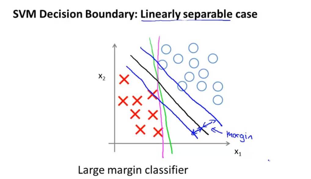
假如我们有一个数据集是这样的，可以看出，这是线性可分的。但是有时候我们的决策边界就好像图中绿色线或者粉红色线一样，这样的决策边界看起来都不是特别好的选择。支持向量机就会选择黑色这一条决策边界。黑色这条边界相比之前跟正负样本有更大的距离，而这个距离就叫做间距（margin）。这也是为什么我们将支持向量机叫做大间距分类器的原因。

支持向量机模型的做法是，即努力将正样本和负样本用最大的间距分开。

$$min_{\theta} C[\sum_{i=1}^{m}{y^{(i)}}cost_1(\theta^Tx^{(i)})+(1-y^{(i)})cost_0(\theta^Tx^{(i)})]+\frac{1}{2}\sum_{j=1}^{n}{\theta_j^2}$$

当 y=1 时，SVM 希望 $\theta^Tx\geqslant 1$ 。在 y=0 时，SVM 希望 $\theta^Tx \leqslant -1$，对于前面的那一项 A 最小化代价函数，那么最理想当然是为0。所以这就变成了：

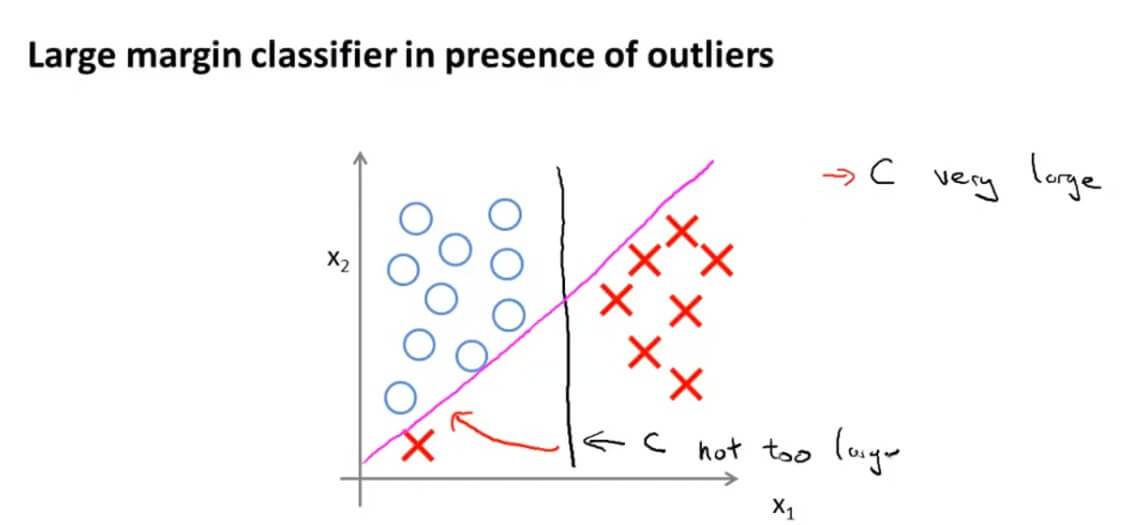
$$min_{\theta}\frac{1}{2}\sum_{i=1}^{n}{\theta_j^2}\;\;\;\;\;\; \left\{\begin{matrix} \theta^Tx\geqslant 1,if \;y^{(i)}=1 \\ \theta^Tx\leqslant 1 ,if \;y^{(i)}=0 \end{matrix}\right. $$

参数 C 其实是支持向量机对异常点的敏感程度，C 越大就越敏感，任何异常点都会影响最终结果。 C 越小，对异常点就越不敏感，普通的一两个异常点都会被忽略。

推导

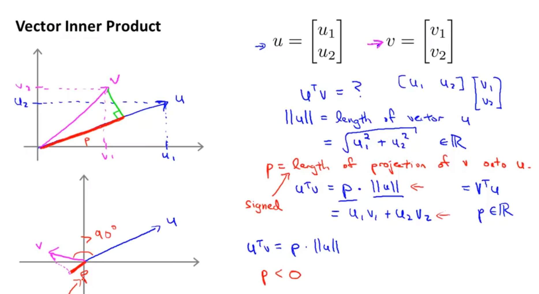
以两个二维向量为例，我们把向量 v 投影到向量 u 上，其投影的长度为 p，$\left \| u \right \|$ 为向量 u 的模，那么向量的内积就等于$p*\left \| u \right \|$。在代数定义向量内积可表示为： $u_1v_1+u_2v_2$ ，根据此定义可以得出： $u^Tv=u_1v_1+u_2v_2$ 。

$\left \| u \right \|$为 $\overrightarrow{u}$ 的范数，也就是向量 $\overrightarrow{u}$ 的欧几里得长度。

最小化函数为： $$min_{\theta}\frac{1}{2}\sum_{i=1}^{n}{\theta_j^2}$$

这里以简单的二维为例：

$$min_{\theta}\frac{1}{2}\sum_{i=1}^{n}{\theta_j^2}=\frac{1}{2}(\theta_1^2+\theta_2^2)=\frac{1}{2}(\sqrt{\theta_1^2+\theta_2^2})^2=\frac{1}{2}\left \| \theta \right \|^2$$

毕达哥拉斯定理：

$$ \left \| u \right \| = \sqrt{u_{1}^{2} + u_{2}^{2}}$$

只要 $\theta$ 能最小，最小化函数就能取到最小。

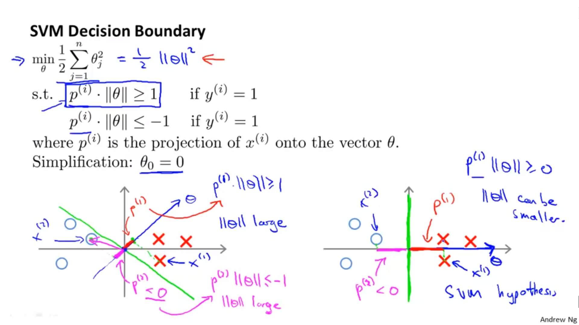
当垂直的时候 $\theta$ 取最小值。这就解释了为什么支持向量机的决策边界不会选择左图绿色那条。因为方便理解所以 $\theta_0=0$ ，这就意味着决策边界要经过原点。然后我们可以看到在垂直于决策边界的 $\theta $和 $x^{(i)}$ 的关系（红色投影和粉红色投影），可以看到其投影 $p^{(i)}$ 的值都比较小，这也就意味着要 $||\theta||^2$ 的值很大。这显然是与最小化公式 $\frac{1}{2}||\theta||^2$ 矛盾的。所以支持向量机的决策边界会使 $p^{(i)}$ 在 $\theta$ 的投影尽量大。这就是为什么决策边界会是右图的原因，也就是为什么支持向量机能有效地产生最大间距分类的原因。

(因为只有最大间距才能使 $p^{(i)}$ 大，从而 $||\theta||^2$ 值小)

三. Kernels

1. 定义

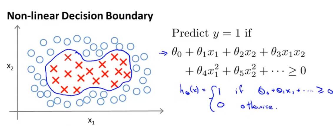
在我们之前拟合一个非线性的判断边界来区别正负样本，是构造多项式特征变量。

我们先用一种新的写法来表示决策边界： $\theta_0+\theta_1f_1+\theta_2f_2+\theta_3f_3+\cdots $。我们这里用 $f_i$ 表达新的特征变量。

假如是之前我们所学的决策边界，那么就是： $f_1=x_1 , f_2=x_2 , f_3=x_1x_2 , f_4=x_1^2 ， f_5=x_2^2$ ，等等。但是这样的高阶项作为特征变量并不是我们确定所需要的，而且运算量非常巨大，那么有没有其他更高的特征变量呢？

下面是构造新特征量的一种想法：

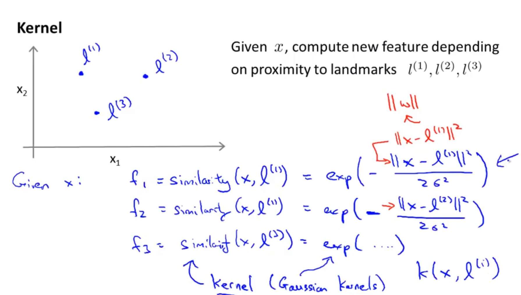
为了简单理解，我们这里只建立三个特征变量。首先我们在 $x_1,x_2$ 坐标轴上手动选择3个不同的点： $l^{(1)},l^{(2)},l^{(3)}$ 。

然后我们将第一个特征量定义为： $f_1=similarity(x,l^{(1)})$ ，可以看做是样本 x 和第一个标记 $l^{(1)}$ 的相似度。其中可以用这个公式表达这种关系： $f_1=similarity(x,l^{(1)})=exp(-\frac{||x-l^{(1)}||^2}{2\sigma^2})$ (exp：自然常数e为底的指数函数)

类似的有： $f_2=similarity(x,l^{(2)})=exp(-\frac{||x-l^{(2)}||^2}{2\sigma^2})$ ，

$f_3=similarity(x,l^{(3)})=exp(-\frac{||x-l^{(3)}||^2}{2\sigma^2})$ 。这个表达式我们称之为核函数（Kernels），在这里我们选用的核函数是高斯核函数（Gaussian Kernels）。

那么高斯核函数与相似性又有什么关系呢？

先来看第一个特征量 $f_1$ ， $f_1=similarity(x,l^{(1)})=exp(-\frac{||x-l^{(1)}||^2}{2\sigma^2})=exp(\frac{\sum_{j=1}^{n}{(x_j-l_j^{(1)})^2}}{2\sigma^2})$

假如样本 x 非常接近 $l^{(1)}$ ，即$x\approx l^{(1)}$ ，那么：$ f_1\approx exp(-\frac{0^2}{2\sigma^2})\approx 1$ 。

假如样本 x 离 $l^{(1)}$ 非常远，即 $x\gg l^{(1)}$ ，那么：$ f_1\approx exp(-\frac{\infty^2}{2\sigma^2})\approx 0$ 。

可视化如下：

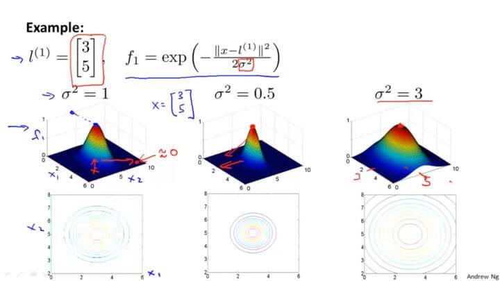
从图中可以看到越接近 $l^{(1)} , f_1$ 的值越大。

这里顺带说一下 $\sigma^2$ 这个高斯核函数的参数对函数的影响。从图中可以看到，减小或者增加只会对图像的肥瘦产生影响，也就是影响增加或者减小的速度而已。

2. 标记点选取

通过标记点以及核函数，训练出非常复杂的非线性判别边界。那标记点 $l^{(1)},l^{(2)},l^{(3)}$ 这些点是怎么来的？

假定我们有如下的数据集：

$$(x^{(1)},y^{(1)}),(x^{(2)},y^{(2)}),(x^{(3)},y^{(3)})\cdots(x^{(m)},y^{(m)})$$

我们就将每个样本作为一个标记点：

$$l^{(1)}=x^{(1)},l^{(2)}=x^{(2)},l^{(3)}=x^{(3)}\cdots l^{(m)}=x^{(m)}$$

则对于样本 $(x^{(i)},y^{(i)})$ ，我们计算其与各个标记点的距离：

$$ \begin{matrix} f^{(i)}_1=sim(x^{(i)},l^{(1)})\\ f^{(i)}_2=sim(x^{(i)},l^{(2)})\\ \vdots \\ f^{(i)}_m=sim(x^{(i)},l^{(3)})\\ \end{matrix} $$

得到新的特征向量： $f \in \mathbb{R}^{m+1} $

$$f = \begin{bmatrix} f_0\\ f_1\\ f_2\\ \vdots \\ f_m \end{bmatrix} $$

其中 $f_0=1$

则具备核函数的 SVM 的训练过程如下：

$$min_{\theta} C[\sum_{i=1}^{m}{y^{(i)}}cost_1(\theta^Tf^{(i)})+(1-y^{(i)})cost_0(\theta^Tf^{(i)})]+\frac{1}{2}\sum_{j=1}^{n}{\theta_j^2}$$

四. SVMs in Practice

1. 使用流行库

作为当今最为流行的分类算法之一，SVM 已经拥有了不少优秀的实现库，如 libsvm 等，因此，我们不再需要自己手动实现 SVM（要知道，一个能用于生产环境的 SVM 模型并非课程中介绍的那么简单）。

在使用这些库时，我们通常需要声明 SVM 需要的两个关键部分：

参数 C
核函数（Kernel）

由于 C 可以看做与正规化参数 $\lambda $ 作用相反，则对于 C 的调节：

低偏差，高方差，即遇到了过拟合时：减小 C 值。
高偏差，低方差，即遇到了欠拟合时：增大 C 值。

而对于核函数的选择有这么一些 tips：

当特征维度 n 较高，而样本规模 m 较小时，不宜使用核函数，否则容易引起过拟合。
当特征维度 n 较低，而样本规模 m 足够大时，考虑使用高斯核函数。不过在使用高斯核函数前，需要进行特征缩放（feature scaling）。
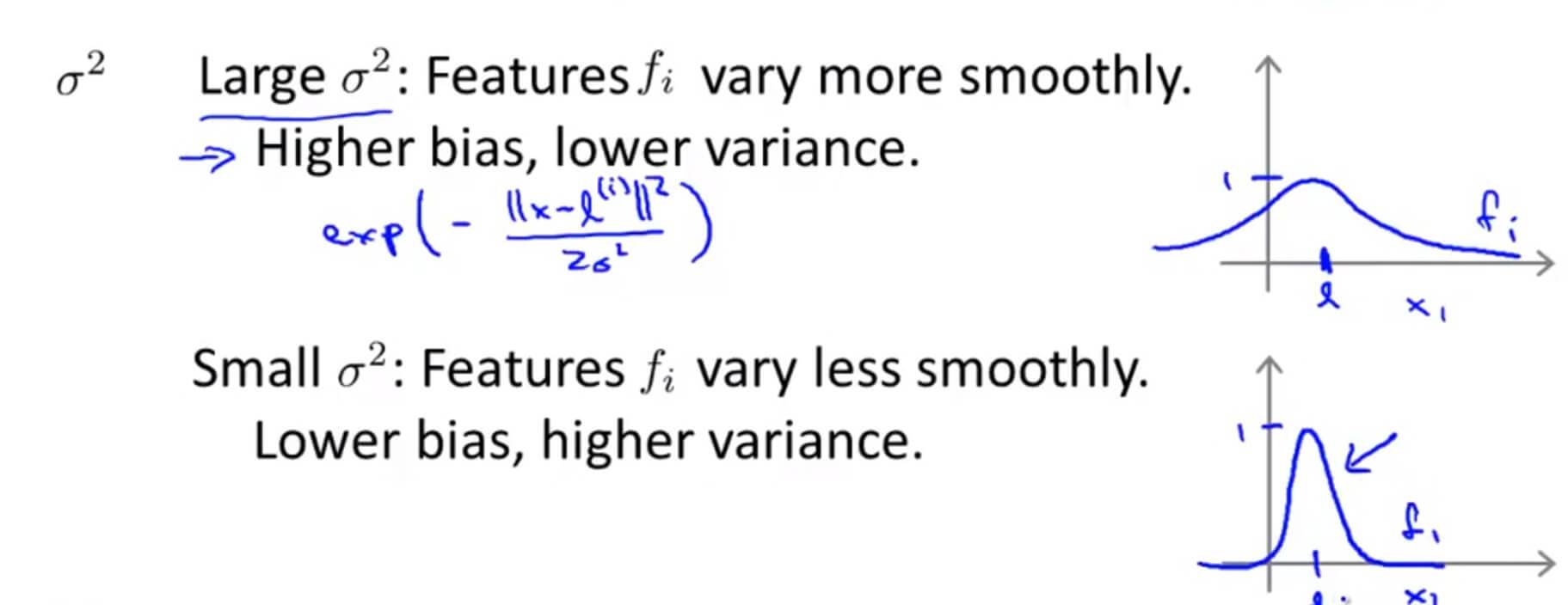
当核函数的参数 $\sigma^2$ 较大时，特征 $f_i$ 较为平缓，即各个样本的特征差异变小，此时会造成欠拟合（高偏差，低方差），如下图上边的图，
当 $\sigma^2$ 较小时，特征 $f_i$ 曲线变化剧烈，即各个样本的特征差异变大，此时会造成过拟合（低偏差，高方差），如下图下边的图：

2. 多分类问题

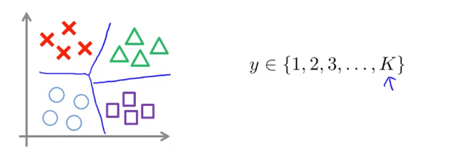
通常，流行的SVM库已经内置了多分类相关的 api，如果其不支持多分类，则与逻辑回归一样，使用 One-vs-All 策略来进行多分类：

轮流选中某一类型 i ，将其视为正样本，即 “1” 分类，剩下样本都看做是负样本，即 “0” 分类。
训练 SVM 得到参数 $\theta^{(1)},\theta^{(2)},\cdots,\theta^{(K)}$ ，即总共获得了 K−1 个决策边界。

3. 分类模型的选择

目前，我们学到的分类模型有：

（1）逻辑回归；
（2）神经网络；
（3）SVM

怎么选择在这三者中做出选择呢？我们考虑特征维度 n 及样本规模 m ：

如果 n 相对于 m 非常大，例如 n=10000 ，而 $m\in(10,1000)$ ：此时选用逻辑回归或者无核的 SVM。

如果 n 较小，m 适中，如 $n\in(1,1000)$ ，而 $m\in(10,10000)$ ：此时选用核函数为高斯核函数的 SVM。

如果 n 较小，m 较大，如 $n\in(1,1000)$ ，而 m>50000 ：此时，需要创建更多的特征（比如通过多项式扩展），再使用逻辑回归或者无核的 SVM。神经网络对于上述情形都有不错的适应性，但是计算性能上较慢。

四. Support_Vector_Machines 测试

1. Question 1

Suppose you have trained an SVM classifier with a Gaussian kernel, and it learned the following decision boundary on the training set:

When you measure the SVM's performance on a cross validation set, it does poorly. Should you try increasing or decreasing C? Increasing or decreasing $\sigma^{2}$?

A. It would be reasonable to try decreasing C. It would also be reasonable to try increasing $\sigma^{2}$.

B. It would be reasonable to try increasing C. It would also be reasonable to try increasing $\sigma^{2}$.

C. It would be reasonable to try increasing C. It would also be reasonable to try decreasing $\sigma^{2}$.

D. It would be reasonable to try decreasing C. It would also be reasonable to try decreasing $\sigma^{2}$.

解答：A

过拟合应该减小 C 和增大 $\sigma^2$

2. Question 2

The formula for the Gaussian kernel is given by similarity $(x,l^{(1)})=exp(-\frac{\left \| x-l^{(1)} \right \|^{2}}{2\sigma^{2} })$ .

The figure below shows a plot of f1=similarity $(x,l^{(1)})$ when $\sigma^{2} = 1$.

Which of the following is a plot of f1 when $\sigma^{2} = 0.25$?

解答：A

$\sigma^{2} $ 变小图像变瘦高。

3. Question 3

The SVM solves

$$min_{\theta} C \sum^{m}_{i=1}y^{(i)}cost_{1}(\theta^{T}x^{(i)})+(1-y^{(i)})cost_{0}(\theta^{T}x^{(i)})+\sum^{n}_{j=1}\theta^{2}_{j}$$

where the functions $cost_0(z)$ and $cost_1(z)$ look like this:

The first term in the objective is:

$$C \sum^{m}_{i=1}y^{(i)}cost_{1}(\theta^{T} x^{(i)})+(1-y^{(i)})cost_{0}(\theta^{T}x^{(i)})$$

This first term will be zero if two of the following four conditions hold true. Which are the two conditions that would guarantee that this term equals zero?

A. For every example with $y^{(i)}=0$, we have that $\theta^{T}x(i) \leqslant 0$.

B. For every example with $y^{(i)}=1$, we have that $\theta^{T}x(i) \geqslant 0$.

C. For every example with $y^{(i)}=0$, we have that $\theta^{T}x(i)\leqslant-1$.

D. For every example with $y^{(i)}=1$, we have that $\theta^{T}x(i)\geqslant 1$.

解答：C、D

4. Question 4

Suppose you have a dataset with n = 10 features and m = 5000 examples.

After training your logistic regression classifier with gradient descent, you find that it has underfit the training set and does not achieve the desired performance on the training or cross validation sets.

Which of the following might be promising steps to take? Check all that apply.

A. Try using a neural network with a large number of hidden units.

B. Create / add new polynomial features.

C. Reduce the number of examples in the training set.

D. Use a different optimization method since using gradient descent to train logistic regression might result in a local minimum.

解答： A、B

题干中要求解决欠拟合的问题。

A.增多神经网络的隐藏层可以解决欠拟合问题。
B.增加特征量可以解决欠拟合问题。
C.减少训练集样本，不行。
D.不是梯度下降函数到达最低值是代价函数。

5. Question 5

Which of the following statements are true? Check all that apply.

A. Suppose you have 2D input examples (ie, $x^{(i)} \in \mathbb{R}^2$). The decision boundary of the SVM (with the linear kernel) is a straight line.

B. If the data are linearly separable, an SVM using a linear kernel will return the same parameters $\theta$ regardless of the chosen value of C (i.e., the resulting value of $\theta$ does not depend on C).

C. If you are training multi-class SVMs with the one-vs-all method, it is not possible to use a kernel.

D. The maximum value of the Gaussian kernel (i.e., $sim(x,l^{(1)})$) is 1.

解答：A、D

A. 线性是一条直线。
B. $min_{\theta} C[\sum_{i=1}^{m}{y^{(i)}}cost_1(\theta^Tx^{(i)})+(1-y^{(i)})cost_0(\theta^Tx^{(i)})]+\frac{1}{2}\sum_{j=1}^{n}{\theta_j^2}$， $\theta$正是由 C 的大小决定的。
C. 解决多分类问题可以用 SVM 。
D. 高斯核函数范围：[0,1]。

GitHub Repo：Halfrost-Field

Follow: halfrost · GitHub

Source: https://github.com/halfrost/Halfrost-Field/blob/master/contents/Machine_Learning/Support_Vector_Machines.ipynb

Tags

初探支持向量机

一. 引子

二. Large Margin Classification 大间距分类器

推导