一. Backpropagation in Practice
为了利用梯度下降的优化算法,需要用到 fminunc 函数。其输入的参数是 $\theta$ ,函数的返回值是代价函数 jVal 和导数值 gradient。然后将返回值传递给高级优化算法 fminunc,然后输出为输入值 @costFunction,以及 $\theta$ 值的初始值。
其中参数 $\Theta_1,\Theta_2,\Theta_3,\cdots$ 和 $D^{(1)},D^{(2)},D^{(3)},\cdots$ 都为矩阵,那么为了能调用 fminunc 函数,我们要将其变成向量,
假如我们 $\Theta_1,\Theta_2,\Theta_3$ 参数和 $D^{(1)},D^{(2)},D^{(3)}$ 参数,Theta1 是 $10 * 11$,Theta2 是 $10 * 11$,Theta3 是 $1 * 11$。
% 打包成一个向量
thetaVector = [ Theta1(:); Theta2(:); Theta3(:); ]
deltaVector = [ D1(:); D2(:); D3(:) ]

% 解包还原
Theta1 = reshape(thetaVector(1:110),10,11)
Theta2 = reshape(thetaVector(111:220),10,11)
Theta3 = reshape(thetaVector(221:231),1,11)
所以套路是:
-
先将 $\Theta_1,\Theta_2,\Theta_3$ ,这些矩阵展开为一个长向量赋值给 initialTheta,然后作为theta参数的初始设置传入优化函数 fminunc。
-
再实现代价函数 costFunction。costFunction 函数将传入参数 thetaVec(就是刚才包含所有 $\Theta$ 参数的向量),然后通过 reshape 函数得到初始的矩阵,这样可以更方便地通过前向传播和反向传播以求得导数 $D^{(1)},D^{(2)},D^{(3)}$ 和代价函数 $F(\Theta)$ 。
-
最后按顺序展开得到 gradientVec,让它们保持和之前展开的 $\theta$ 值同样的顺序。以一个向量的形式返回这些导数值。
二. Gradient Checking
在计算导数的时候,习惯将其等于在该点的导数,在我们使用梯度下降计算导数的时候,虽然可能 $F(\Theta)$ 每次迭代都在下降,但是因为反向传播的复杂性,可能导致我们的代码存在 BUG。有一个办法叫做梯度检验(Gradient Checking),它能减少这种错误的概率(出现这个问题的原因都和反向传播的错误实现有关)。
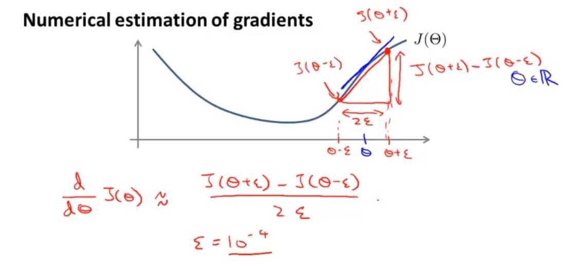
在我们求该点的斜率的时候,我们不直接使用其导数,而是用 $$\frac{d}{d\Theta}F(\Theta)\approx\frac{F(\Theta+\epsilon)-F(\Theta-\epsilon)}{2\epsilon}$$ 代替。通常 $\epsilon$ 取较小的一个数。(其实就是使用导数的定义)
上面这种算法是双侧差分算法,与之相对的是单侧差分算法
$$\frac{d}{d\Theta}F(\Theta)\approx\frac{F(\Theta+\epsilon)-F(\Theta)}{\epsilon}$$
单侧差分和双侧差分相比,双侧差分可以得到更加准确的结果。
推广一下双侧差分:
$$\frac{d}{d\Theta_j}J(\Theta)\approx\frac{J(\Theta_1,…,+\Theta_j+\epsilon,…,\Theta_n)-J(\Theta_1,…,+\Theta_j-\epsilon,…,\Theta_n)}{2\epsilon}$$
对应代码实现如下:
epsilon = 1e-4;
for i = 1:n,
  thetaPlus = theta;
  thetaPlus(i) += epsilon;
  thetaMinus = theta;
  thetaMinus(i) -= epsilon;
  gradApprox(i) = (J(thetaPlus) - J(thetaMinus))/(2*epsilon)
end;
检查反向传播计算出来的导数 DVec 和 上面程序计算出来的 gradApprox 相比较,如果 $gradApprox \approx DVec$ 代表反向传播的实现是正确的。
最后在使用算法学习的时候关闭梯度检验。因为梯度检验主要是为了让我们知道我们写的程序算法是否存在错误,而不是用来计算导数的,因为这种方法计算导数相比于之前的会非常慢。
总结一下:
- 通过反向传播来计算 DVec,DVec 是每个矩阵打包展开的形式。
- 实现数值上的梯度检测,计算出 gradApprox。
- 比较 $gradApprox \approx DVec$ 是否相等或者约等于。
- 使用算法学习的时候记得要关闭这个梯度检验,梯度检验只在代码测试阶段进行。
三. Random Initialization
使用梯度下降算法的时候,需要设置 $\Theta$ 初始值。
optTheta = fminunc(@costFunction, initialTheta, options)
调用 fminunc 函数的时候,initialTheta 如果全部初始化为0,
initialTheta = zeros(n,1)
在之前的线性回归和逻辑回归中,使用梯度函数,初始值设置为0是没有问题的,但是到了神经网络里面,如果还这么设置,会出现高度冗余现象。
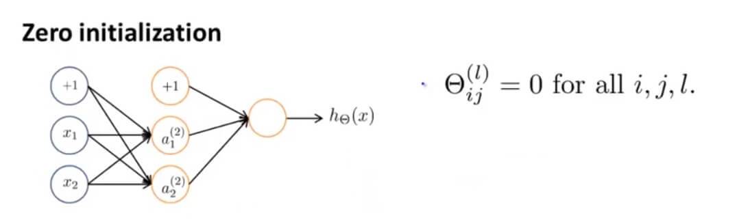
假设我们有这样一个网络,其初始参数都设为0。那么我们会发现其激励 $a_1^{(2)}=a_2^{(2)}$ ,且误差 $\delta_1^{(2)}=\delta_2^{(2)}$ ,且导数 $\frac{d}{d\Theta^{(1)}_{01}}J(\Theta)=\frac{d}{d\Theta^{(1)}_{02}}J(\Theta)$ 。这就导致了在参数更新的情况下,两个参数是一样的。无论怎么重复计算其两边的激励还是一样的。
上述问题被称为,对称权重问题,也就是所有权重都是一样的。所以随机初始化是解决这个问题的方法。
我们将初始化权值 $\Theta_{ij}^{(l)}$ 的范围限定在 $[-\Phi ,\Phi ]$ 。
其代码表示如下:
%If the dimensions of Theta1 is 10x11, Theta2 is 10x11 and Theta3 is 1x11.

Theta1 = rand(10,11) * (2 * INIT_EPSILON) - INIT_EPSILON;
Theta2 = rand(10,11) * (2 * INIT_EPSILON) - INIT_EPSILON;
Theta3 = rand(1,11) * (2 * INIT_EPSILON) - INIT_EPSILON;
rand(x,y)是随机函数,它将初始化一个0到1之间的随机实数矩阵。
四. 总结
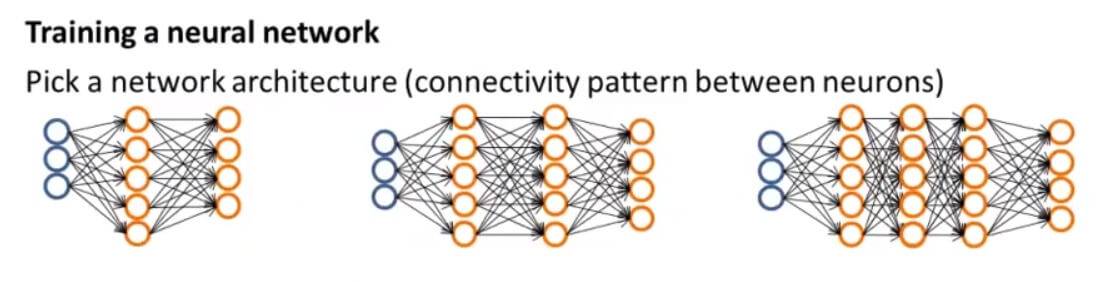
1. 准备
首先,我们需要确定神经网络有多少输入单元,有多少隐藏层,每一层隐藏层又有多少个单元,还有多少输出单元。那我们怎么去选择呢?
- 输入单元是特征向量 $x^{(i)}$ 的维度
- 输出单元是分类的个数
- 每个隐藏层的单元数通常是越多越好(必须与计算成本平衡,因为随着更多隐藏单元的增加而增加)
- 默认值:1个隐藏层。如果有多个隐藏层,那么建议您在每个隐藏层中都有相同数量的单元。
输出单元如果是多元分类问题,输出单元需要写成矩阵的形式:
例如有3个分类, 输出单元应该写成
2. 训练
第一步:随机初始化权重。初始化的值是随机的,值很小,接近于零。
第二步:执行前向传播算法,对于每一个 $x^{(i)}$ 计算出假设函数 $h_\Theta(x^{(i)})$ 。
第三步:计算出代价函数 $F(\Theta)$ 。
第四步:执行反向传播算法,计算出偏导数 $\frac{\partial}{\partial\Theta_{jk}^{(l)}}F(\Theta)$ 。
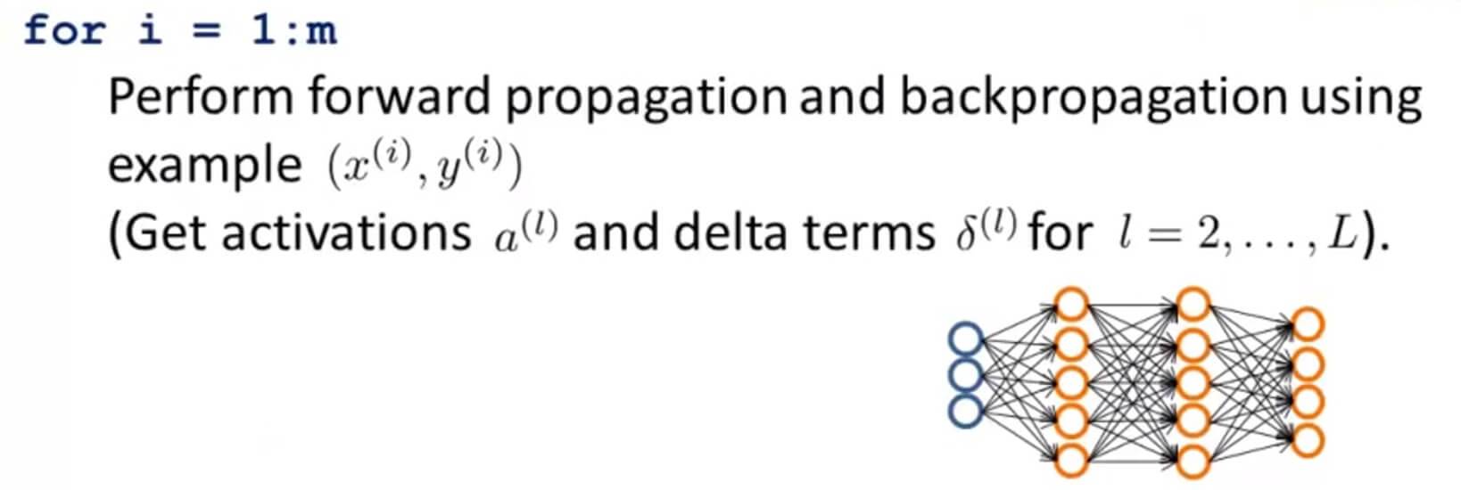
具体操作就是使用一个for循环,先将 $(x^{(1)},y^{(1)})$ 进行一次前向传播和后向传播的操作,然后再对 $(x^{(2)},y^{(2)})$ 进行相同的操作一直到 $(x^{(n)},y^{(n)})$ ,这样就能得到神经网络中每一层中每个单元对应的激励值,和每一层激励的误差 $\delta^{(l)}$ 。
第五步:利用梯度检查,对比反向传播算法计算得到的偏导数项是否与梯度检验算法计算出的导数项基本相等。检查完记得删除掉这段检查的代码。
第六步:最后我们利用梯度下降算法或者更高级的算法例如 LBFGS、共轭梯度法等,结合之前算出的偏导数项,最小化代价函数 $F(\Theta)$ 算出权值的大小 $\Theta$ 。
理想情况下,只要满足了 $h_{\Theta}(x^{(i)})\approx y^{(i)}$,就能使我们的代价函数最小。但是,代价函数 $F(\Theta)$ 不是凸的,因此我们最终可以用局部最小值代替全局最小值。
五. Neural Networks: Learning 测试
1. Question 1
You are training a three layer neural network and would like to use backpropagation to compute the gradient of the cost function. In the backpropagation algorithm, one of the steps is to update
$\Delta^{(2)}_{ij}:=\Delta^{(2)}_{ij}+\delta^{(3)}_{i}*(a^{(2)})_{j}$
for every i,j. Which of the following is a correct vectorization of this step?
A. $\Delta^{(2)}:=\Delta^{(2)}+(a^{(3)})^T * \delta^{(2)} $
B. $\Delta^{(2)}:=\Delta^{(2)}+(a^{(2)})^T * \delta^{(3)} $
C. $\Delta^{(2)}:=\Delta^{(2)}+\delta^{(3)} * (a^{(3)})^T $
D. $\Delta^{(2)}:=\Delta^{(2)}+\delta^{(3)} * (a^{(2)})^T $
解答: D
2. Question 2
Suppose Theta1 is a 5x3 matrix, and Theta2 is a 4x6 matrix. You set thetaVec=[Theta1(:);Theta2(:)]. Which of the following correctly recovers Theta2?
A. reshape(thetaVec(16:39),4,6)
B. reshape(thetaVec(15:38),4,6)
C. reshape(thetaVec(16:24),4,6)
D. reshape(thetaVec(15:39),4,6)
E. reshape(thetaVec(16:39),6,4)
解答:A
3. Question 3
Let $J(\theta)=2\theta^3+2$ . Let $\theta=1$ , and $\epsilon=0.01$ . Use the formula $\frac{J(\theta+\epsilon)-J(\theta-\epsilon)}{2\epsilon}$ to numerically compute an approximation to the derivative at $\theta=1$ . What value do you get? (When $\theta=1$ , the true/exact derivati ve is $\frac{dJ(\theta)}{d\theta}=6$ .)
A.6
B.8
C.5.9998
D.6.0002
解答: D
4. Question 4
Which of the following statements are true? Check all that apply.
A. Gradient checking is useful if we are using gradient descent as our optimization algorithm. However, it serves little purpose if we are using one of the advanced optimization methods (such as in fminunc).
B. If our neural network overfits the training set, one reasonable step to take is to increase the regularization parameter λ .
C. Using gradient checking can help verify if one's implementation of backpropagation is bug-free.
D. Using a large value of λ cannot hurt the performance of your neural network; the only reason we do not set λ to be too large is to avoid numerical problems.
E. For computational efficiency, after we have performed gradient checking to verify that our backpropagation code is correct, we usually disable gradient checking before using backpropagation to train the network.
F. Computing the gradient of the cost function in a neural network has the same efficiency when we use backpropagation or when we numerically compute it using the method of gradient checking.
解答:B、C、E
A.梯度检验只是用来检验我们算偏导数的算法是否正确,而不是用来计算的。
B.过拟合增大正则化参数 λ 正确。
C.梯度检验能检验反向传播算法是否正确。
D.正则化参数 λ 太大会导致欠拟合。
E.还是在说梯度检验能验证反向传播算法的正确性。
F.还是在说梯度检验可以用来在算法里算偏导数。
5. Question 5
Which of the following statements are true? Check all that apply.
A. Suppose you have a three layer network with parameters $\Theta^{(1)}$ (controlling the function mapping from the inputs to the hidden units) and $\Theta^{(2)}$ (controlling the mapping from the hidden units to the outputs). If we set all the elements of $\Theta^{(1)}$ to be 0, and all the elements of $\Theta^{(2)}$ to be 1, then this suffices for symmetry breaking, since the neurons are no longer all computing the same function of the input.
B. If we are training a neural network using gradient descent, one reasonable "debugging" step to make sure it is working is to plot $J(\Theta)$ as a function of the number of iterations, and make sure it is decreasing (or at least non-increasing) after each iteration.
C. Suppose you are training a neural network using gradient descent. Depending on your random initialization, your algorithm may converge to different local optima (i.e., if you run the algorithm twice with different random initializations, gradient descent may converge to two different solutions).
D. If we initialize all the parameters of a neural network to ones instead of zeros, this will suffice for the purpose of "symmetry breaking" because the parameters are no longer symmetrically equal to zero.
E. If we are training a neural network using gradient descent, one reasonable "debugging" step to make sure it is working is to plot $J(\Theta)$ as a function of the number of iterations, and make sure it is decreasing (or at least non-increasing) after each iteration.
F. Suppose we have a correct implementation of backpropagation, and are training a neural network using gradient descent. Suppose we plot $J(\Theta)$ as a function of the number of iterations, and find that it is increasing rather than decreasing. One possible cause of this is that the learning rate $\alpha$ is too large.
G. Suppose that the parameter $\Theta^{(1)}$ is a square matrix (meaning the number of rows equals the number of columns). If we replace $\Theta^{(1)}$ with its transpose $(\Theta^{(1)})^T$ , then we have not changed the function that the network is computing.
H. Suppose we are using gradient descent with learning rate $\alpha$ . For logistic regression and linear regression, $J(\Theta)$ was a convex optimization problem and thus we did not want to choose a learning rate $\alpha$ that is too large. For a neural network however, $J(\Theta)$ may not be convex, and thus choosing a very large value of $\alpha$ can only speed up convergence.
解答:B、C、F
A.一层的权重都是一样的数字不能打破对称。
B.迭代次数的越多,代价函数 $J(\Theta)$ 下降正确。
C.学习速率 $\alpha$ 太大会导致代价函数随着迭代次数的增加也增加正确。
D.权重全部为1也不能打破对称的。
E.保证 $J(\Theta)$ 随着迭代次数的增加而下降用以验证算法的正确。
F.同B。
G.矩阵的倒置一般不相等。
H.选择大的学习速率 $\alpha$ 会导致 $J(\Theta)$ 不收敛的。
GitHub Repo:Halfrost-Field
Follow: halfrost · GitHub